PyNNDescent Performance
How fast is PyNNDescent for approximate nearest neighbor search? How does it compare with other approximate nearest neighbor search algorithms and implementations? To answer these kinds of questions we’ll make use of the ann-benchmarks suite of tools for benchmarking approximate nearest neighbor (ANN) search algorithms. The suite provides a wide array of datasets to benchmark on, and supports a wide array of ANN search libraries. Since the runtime of these benchmarks is quite large we’ll be presenting results obtained earlier, and only for a selection of datasets and for the main state-of-the-art implementations. This page thus reflects the performance at a given point in time, and on a specific choice of benchmarking hardware. Implementations may (and likely will) improve, and different hardware will likely result in somewhat different performance characteristics amongst the implementations benchmarked here.
We chose the following implementations of ANN search based on their strong performance in ANN search benchmarks in general:
Annoy (a tree based algorithm for comparison)
HNSW from FAISS, Facebooks ANN library
HNSW from nmslib, the reference implementation of the algorithm
HNSW from hnswlib, a small spinoff library from nmslib
ONNG from NGT, a more recent algorithm and implementaton with impressive performance
PyNNDescent version 0.5
Not all the algorithms ran entirely successfully on all the datasets; where an algorithm gave spurious or unrepresentative results we have left it off rather the given benchmark.
The ann-benchmark suite is designed to look at the trade-off in performance between search accuracy and search speed (or other performance statistic, such as index creation time, or index size). Since this is a trade-off that can often be tuned by appropriately adjusting parameters ann-benchmarks handles this by running a predefined (for each algorithm or implementation) range of parameters. It then finds the pareto frontier for the optimal speed / accuracy trade-off and presents this as a curve. The various implementations can then be compared in terms of the pareto frontier curves. The default choices of measure for ann-benchmarks puts recall (effective search accuracy) along the x-axis and queries-per-second (search speed) on the y-axis. Thus curves that are further up and / or more to the right are providing better speed and / or more accuracy.
To get a good overview of the relative performance characteristics of the different implementations we’ll look at the speed / accuracy trade-off curves for a variety of datasets. This is because the dataset size, dimensionality, distribution and metric can all have non-trivial impacts on performance in various ways, and results for one dataset are not necessarily representative of how things will look for a different dataset. We will introduce each dataset in turn, and then look at the performance curves. To start with we’ll consider datasets which use Euclidean distance.
Euclidean distance
Euclidean distance is the usual notion of distance that we are familiar with in everyday life, just extended to arbitrary dimensions (instead of only two or three). It is defined as \(d(\bar{x}, \bar{y}) = \sum_i (x_i - y_i)^2\) for vectors \(\bar{x} = (x_1, x_2, \ldots, x_D)\) and \(\bar{y} = (y_1, y_2, \ldots, y_D)\). It is widely used as a distance measure, but can have difficulties with high dimensional data in some cases.
The first dataset we will consider that uses Euclidean distance is the MNIST dataset. MNIST consists of grayscale images of handwritten digits (from 0 to 9). Each digit image is 28 by 28 pixels, which is usually unravelled into a single vectors of 784 dimensions. In total there are 70,000 images in the dataset, and ann-benchmarks uses the usual split into 60,000 training samples and 10,000 test samples. The ANN index is built on the training set, and then the test set is used as the query data for benchmarking.
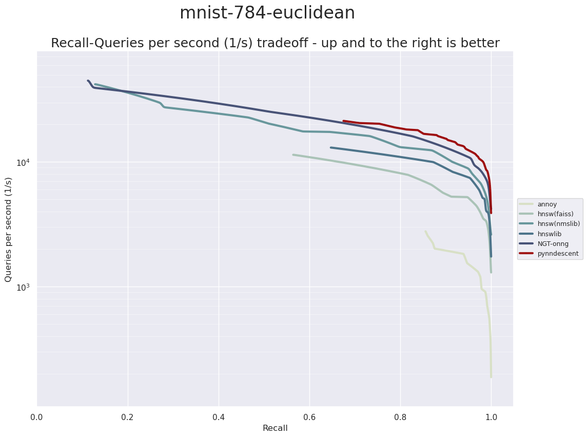
Remember that up and to the right is better. Also note that the y axis (queries per second) is plotted in log scale so each major grid step represents an order of magnitude performance difference. We can see that PyNNDescent performs very well here, outpacing the other ANN libraries in the high accuracy range. It is worth noting, however, that for lower accuracy queries it finishes essentially on par with ONNG, and unlike ONNG and nmslib’s HNSW implementation, it does not extend to very high performance but low accuracy queries. If speed is absolutely paramount, and you only need to be in the vaguely right ballpark for accuracy then PyNNDescent may not be the right choice here.
Next up for dataset is Fashion-MNIST. This was a dataset designed to be a drop in replacement for MNIST, but meant to be more challenging for machine learning tasks. Instead of grayscale images of digits it is grayscale images of fashion items (dresses, shirts, pants, boots, sandas, handbags, etc.). Just like MNIST each image is 28 by 28 pixels resulting in 784-dimensional vectors. Also just like MNIST there are 70,000 total images, split into 60,000 training images and 10,000 test images.
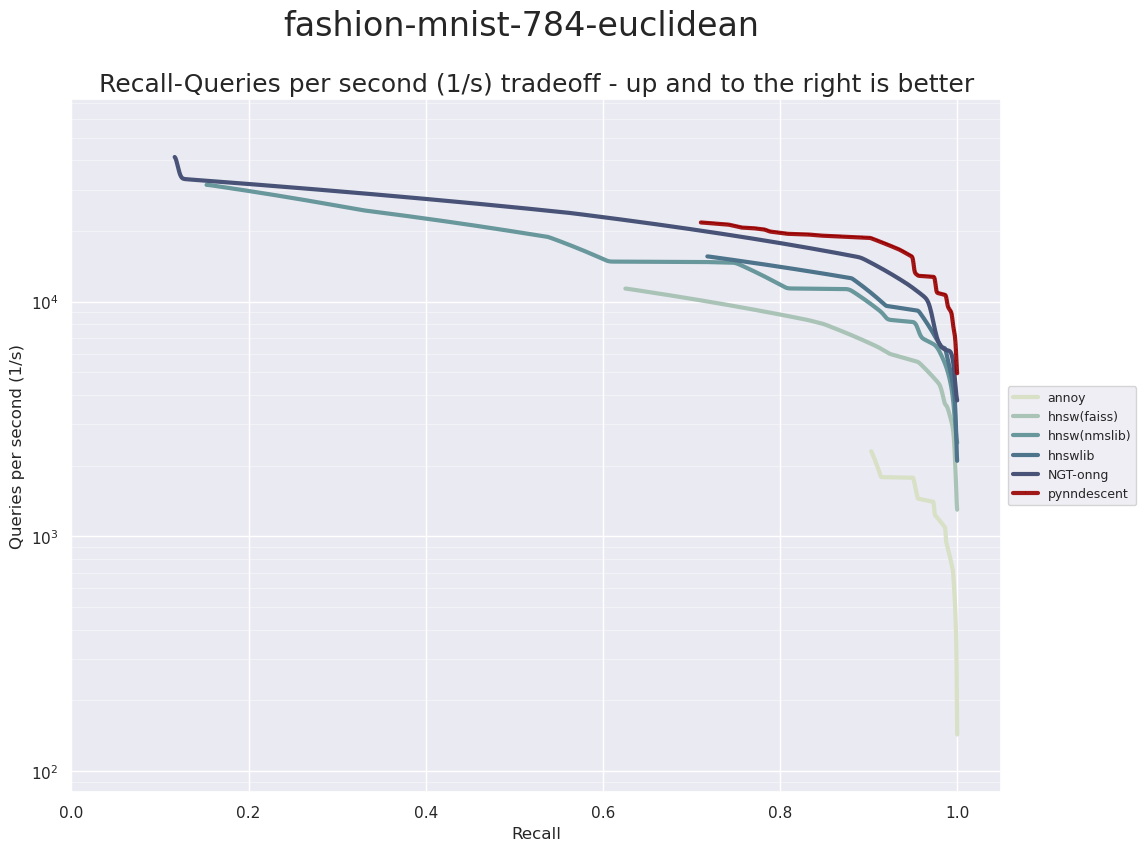
Again we see a very similar result (although this should not entirely be a surprise given the similarity of the dataset in terms of the number of samples and dimensionality). PyNNDescent performs very well in the high accuracy regime, but does not scale to the very high performance but low accuracy ranges that ONNG and nmslib’s HNSW manage. It is also worth noting the clear difference between the various graph based search algorithms and the tree based Annoy – while Annoy is a very impressive ANN search implementation it compares poorly to the graph based search techniques on these datasets.
Next up is the SIFT dataset. SIFT stands for Scale-Invariant Feature Transform and is a technique from compute vision for generating feature vectors from images. For ann-benchmarks this means that there exist some large databases of SIFT features from image datasets which can be used to test nearest neighbor search. In particular the SIFT dataset in ann-benchmarks is a dataset of one million SIFT vectors where each vector is 128-dimensional. This provides a good contrast to the earlier datasets which had relatively high dimensionality, but not an especially large number of samples. For ann-benchmarks the dataset is split into 990,000 training samples, and 10,000 test samples for querying with.

Again we see that PyNNDescent performs very well. This time, however, with the more challenging search problem presented by a training set this large, it does produce some lower accuracy searches and in those cases both ONG and nmslib’s HNSW outperform it. It’s also worth noting that in this lower dimensional dataset Annoy performs better, comparatively, than the previous datasets. Still, over the Euclidean distance datasets tested here PyNNDescent remains a clear winner for high accuracy queries. Let’s move on to the angular distance based datasets.
Angular distance
Angular based distances measure the similarity of two vectors in terms of the angle they span – the greater the angle the larger the distance between the vectors. Thus two vectors of different length can be viewed as being very close as long as they are pointing in the same direction. Another way of looking at this is to imagine that the data is being projected onto a high dimensional sphere (by intersecting a ray in the vectors direction with a unit sphere), and distances are measured in terms of arcs around the sphere.
In practice the most commonly used angular distance is cosine distance, defined as
where \(\|\bar{x}\|_2\) denotes the \(\ell^2\) norm of \(\bar{x}\). To see why this is a measure of angular distance note that \(\sum_i x_i y_i\) is the euclidean dot product of \(\bar{x}\) and \(\bar{y}\) and that the euclidean dot product formula gives \(\bar{x}\cdot \bar{y} = \|x\|_2 \|y\|_2 \cos\theta\) where \(\theta\) is the angle between the vectors.
In the case where the vectors all have unit norm the cosine distance reduces to just one minus the dot product of the vectors – which is sometimes used as an angular distance measure. Indeed, that is the case for our first dataset, the LastFM dataset. This dataset is constructed of 64 factors in a recommendation system for the Last FM online music service. It contains 292,385 training samples and 50,000 test samples. Compared to the other datasets explored so far this is considerably lower dimensional and the distance computation is simpler. Let’s see what results we get.
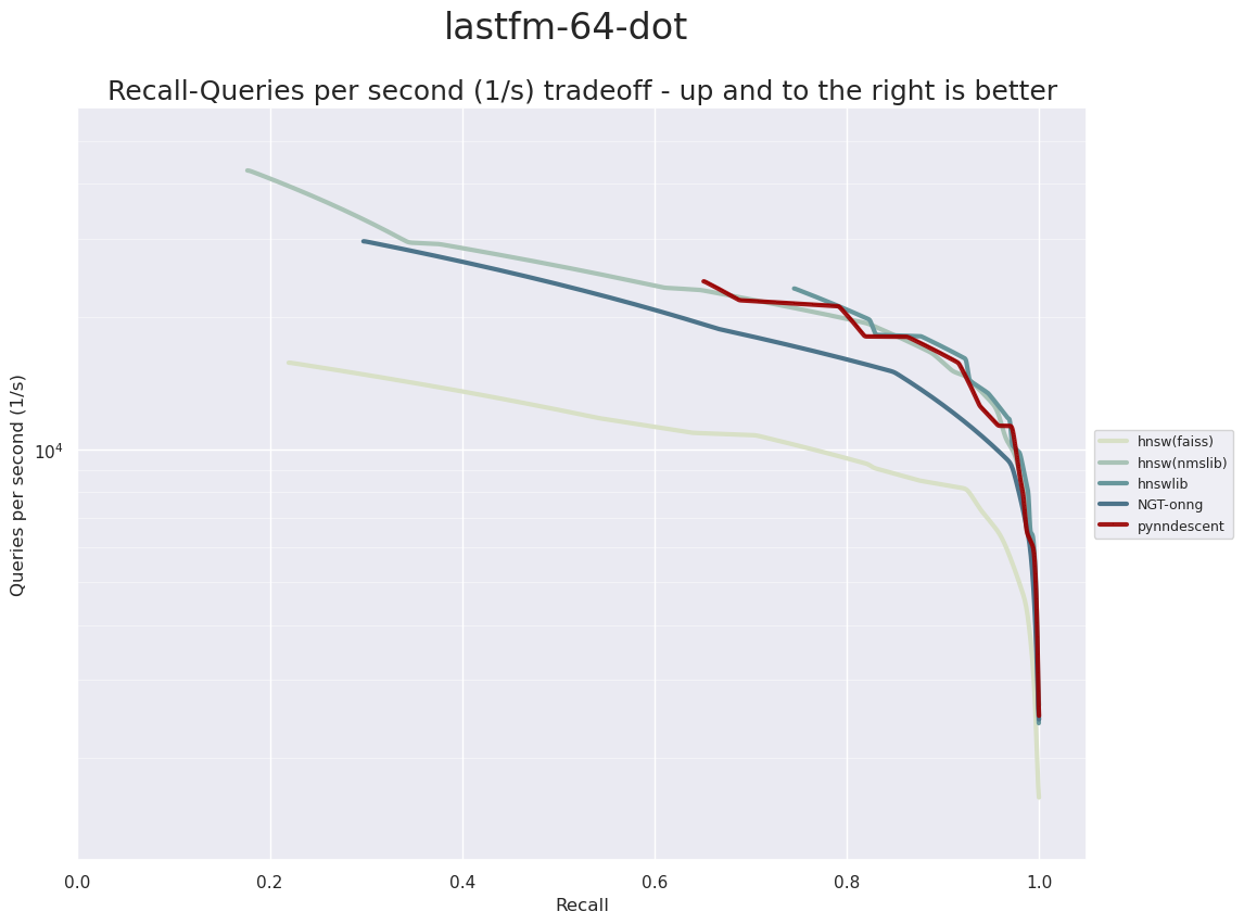
Here we see hnswlib and HNSW from nmslib performing extremely well – outpacing ONNG unlike we saw in the previous euclidean datasets. The HNSW implementation is FAISS is further behind. While PyNNDescent is not the fastest option on this dataset it is highly competitive with the two top performing HNSW implementations.
The next dataset is a GloVe dataset of word vectors. The GloVe datasets are generated from a word-word co-occurrence count matrix generated from vast collections of text. Each word that occurs (frequently enough) in the text will get a resulting vector, with the principle that words with similar meanings will be assigned vectors that are similar (in angular distance). The dimensionality of the generated vectors is an input to the GloVe algorithm. For the first of the the GloVe datasets we will be looking at the 25 dimensional vectors. Since GloVe vectors were trained useing a vast corpus there are over one million different words represented, and thus we have 1,183,514 training samples and 10,000 test samples to work with. This gives is a low dimensional but extremely large dataset to work with.
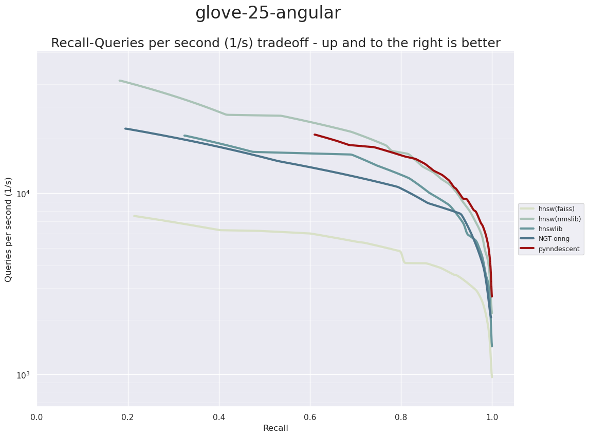
In this case PyNNDescent and hnswlib are the apparent winners – although PyNNDescent, similar to the earlier examples, performs less well once we get below abot 80% accuracy.
Next we’ll move up to a higher dimensional version of GloVe vectors. These vectors were trained on the same underlying text dataset, so we have the same number of samples (both for train and test), but now we have 100 dimensional vectors. This makes the problem more challenging as the underlying distance computation is a little more expensive given the higher dimensionality.
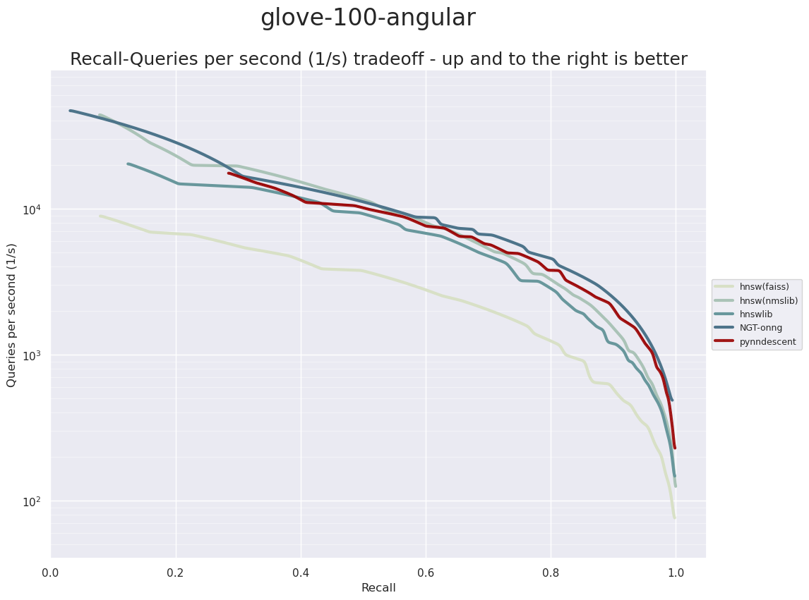
This time it is ONNG that surges to the front of the pack. Relatively speaking PyNNDescent is not too far behind. This goes to show, however, how much performance can vary based on the exact nature of the dataset: while ONNG was a (relatively) poor performer on the 25-dimensional version of this data with hnswlib out in front, the roles are reversed for this 100-dimensional data.
The last dataset is the NY-Times dataset. This is data generated as dimension reduced (via PCA) TF-IDF vectors of New York Times articles. The resulting dataset has 290,000 training samples and 10,000 test samples in 256 dimensions. This is quite a challenging dataset, and all the algorithms have significantly lower query-per-second performance on this data.
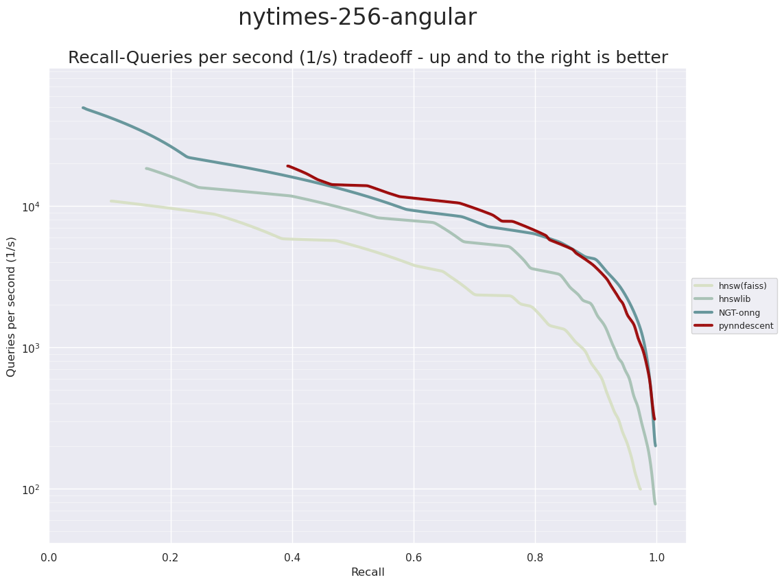
Here we see that PyNNDescent and ONNG are the best performing implementations, particularly at the higher accuracy range (ONNG has a slight edge on PyNNDescent here).
This concludes our examination of performance for now. Having examined performance for many different datasets it is clear that the various algorithms and implementations vary in performance depending on the exact nature of the data. None the less, we hope that this has demonstrated that PyNNDescent has excellent performance characteristics across a wide variety of datasets, often performing better than many state-of-the-art implementations.