How PyNNDescent works
PyNNDescent uses neighbor graph based searching to efficiently find good candidates for the nearest neighbors of query points from a large training set. While the basic ideas turn out to be quite simple, the layers of refinements and tricks used to get the highest degree of efficiency complicate things a lot. With that in mind we will begin with the simple naive approach and gradually work out further refinements and details as we go. The core concept, upon which most everything else is based, is using a nearest neighbor graph to perform a search for approximate nearest neighbors.
Searching using a nearest neighbor graph
Suppose we are given a nearest neighbor graph (let’s ignore, for now, how we can have obtained such a thing without the ability to find nearest neighbors already). By a graph, I simply mean a network – a set of nodes connected by edges. By a nearest neighbor graph I mean that the graph has been derived from data existing in some sort of space for which we have a quantitative notion of similarity, or dissimilarity, or distance. In particular the graph is derived by making each data point a node and connecting that data point, via edges, to the \(k\) most similar, least dissimilar, or closest other points. We would like to use this graph as an index structure for searching to find the nearest neighbors (points in the graph) of a new query point (potentially not a point in the graph) with respect to that notion of similarity of distance. How can we do this? We can do it via a kind of pruned breadth-first search of the graph, always keeping only the \(k\) best points we’ve found so far. The algorithm, therefore, looks something like this:
Choose a starting node in the graph (potentially randomly) as a candidate node
Look at all nodes connected by an edge to the best untried candidate node in the graph
Add all these nodes to our potential candidate pool
Sort the candidate pool by closeness / similarity to the query point
Truncate the pool to \(k\) best (as in closest to the query) candidates
Return to step 2, unless we have already tried all the candidates in the pool
We can see this play out visually on a small graph. For this case we will let \(k=2\) and have a 2-neighbor graph constructed by points in a plane. The query point will be drawn as an orange ‘x’. We then search, exactly as described, and find ourselves steadily traversing the graph towards the query point.
While that did indeed find the points closest to the query point, it was hardly more efficient than a linear search of all the points – there are only two points we didn’t try! This is ultimately about having such a small graph: while it is good for showing the algorithm clearly, the algorithm doesn’t really scale down that well to this case. If we want to see it providing benefits we’ll need a larger graph. That’s not hard to generate, so let’s see a larger example.
Now, with about as bad a start as we could hope to get, the algorithm efficiently traverses across the graph and find the neighbors of the orange query point, and this time we see that only a small fraction of the total number of points in the graph had to be tried. If we had been a little luckier with our start point we could have done significantly better again. We can scale up to even larger examples:
Again we had about as bad a starting point as possible, but again it very efficiently traverses the graph, steadily improving as it goes, until the algorithm eventually find the nearest neighbors of the orange query point. Notably the algorithm will continue to scale well as the number of points increases, and even as the dimension of the data increases – as long as the data itself has a low enough intrisic dimension.
There are, of course, several things that can be done to refine this algorithm to be a little more efficient, and more flexible at the same time. They include such things as keeping a hashtable of visited nodes to ensure you don’t compute distances twice, and keeping a slightly larger priority queue of candidate nodes to expand – anything with (1+\(\varepsilon\)) of the \(k\)th best candidate found so far will suffice. This latter point allows us greater flexibility in search, allowing a degree of backtracking around local “optima” in the search. It also provides a parameter which we can tune to get a trade-off between the speed and accuracy that we desire: smaller epsilon gives a faster search, but less accuracy, while a large epsilon can give good accuracy but at the cost of a slower search.
All of this presumed, however, that we had a nearest neighbor graph to start with – the thing that we were using as our search index. The question remains: how are we to build that, since we could potentially just use the nearest neighbor search technique used to build the graph (which presumably has to be cheap) instead of the graph search described here. The answer, as it happens, is that we are going to use the graph search technique to build the graph itself – pulling ourselves up by our own bootstraps so to speak.
NNDescent for building neighbor graphs
A good way to get to grips with the NNDescent algorithm for constructing approximate k-neighbor graphs is to think of it in terms of the search algorithm we’ve already described. Suppose we had a decent, but not exact, k-neighbor graph. We could use that graph as our search index – it won’t be great, and our search will be particularly approximate and often get stuck in local minima because of that, but it will still work a lot of the time. So, given that graph we could do a nearest neighbor search, using that graph as the index, for each and every point in the dataset. Because of the nature of the search we could end up finding new neighbors for a node that are closer than the ones in our not-so-good graph. We could use that information to update our graph – make it better by using these newly found closer neighbors. Having improved the graph, we can run the search again for each and every point in the dataset. Since the graph is better we will do an even better job of finding neighbors than before and potentially find some new neighbors that will let us update the graph again.
And that’s actually the core of the algorithm. Start with a bad graph, use the nearest neighbor search on that graph to get better neighbors, and make a better graph. Rinse, repeat, and eventually we will end up with a good graph. In fact, the better the graph is, the faster and more accurate the search will run. So each iteration will go faster than the last, and we will steadily converge toward the true k-neighbor graph.
There are a couple things to take note of at this point: a better graph results in a better search, so making a better graph sooner will help the search; finding a good initial candidate node for the search was generically a problem (our animations all had particularly bad initial candidates), but we can always use the point itself as the initial candidate since it is guaranteed to be in the graph. So, given a good initial candidate (the node itself), and a desire to update the graph as soon as possible, it may not be worth running a full search to exhaustion. Instead we could run the search just far enough to potentially find some new neighbors that we haven’t seen before. The first round of search, starting from the node itself, will only find the neighbors we already have. The second round, however, will step out to neighbors of neighbors (friends of friends if you will), and potentially find some nodes that are closer neighbors than the ones currently in the graph. That would be enough information to improve the graph – since we would have found new better neighbors. So the algorithm would now run:
Start with a random graph (connect each node to \(k\) random nodes)
For each node:
Measure the distance from the node to the neighbors of its neighbors
If any are closer then update the graph accordingly, and keep only the \(k\) closest
If any updates were made to the graph then go back to step 2, otherwise stop
We can see this play out on some example data (the same data as the medium sized search example):
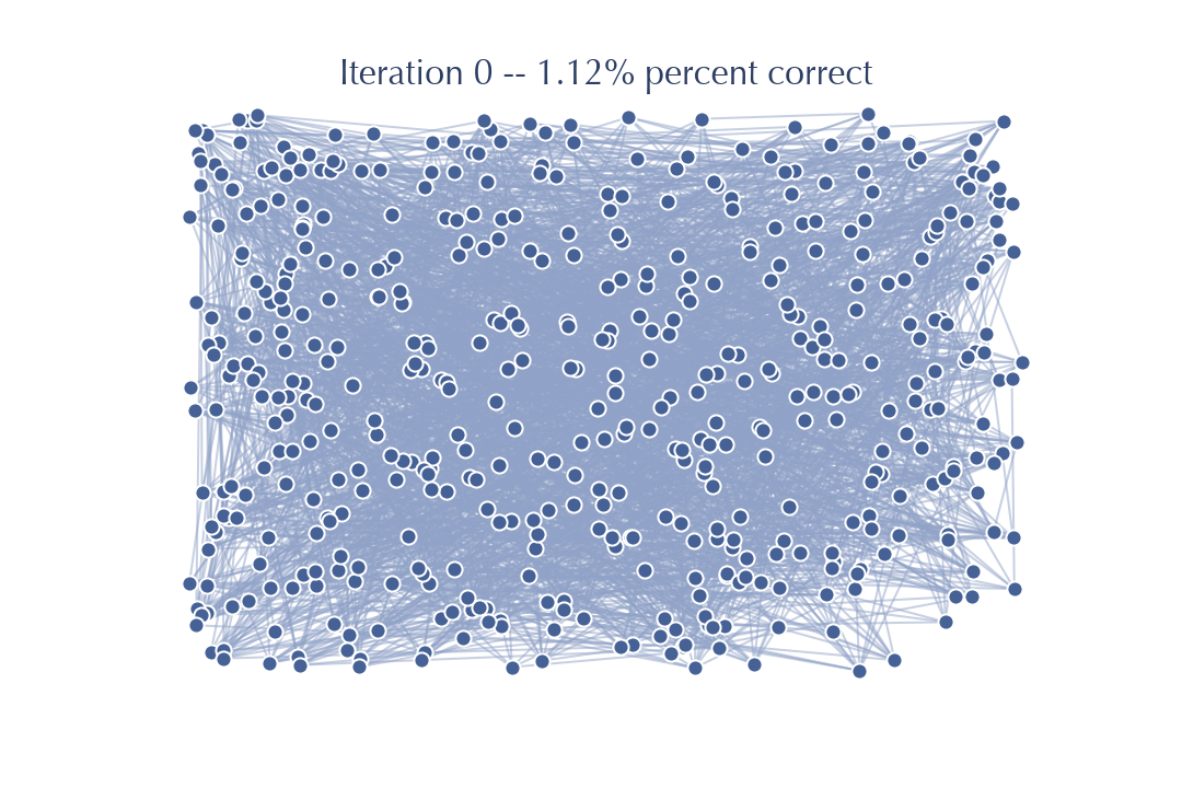
You can see the graph starts out looking nothing like a \(k\)-neighbors graph – just a mess of edges all over with no structure. Quickly, however, we update the graph, and the better the graph gets the better our updates go. After not very long at all the algorithm is simply refining an already very good graph with few, if any, updates at all actually occurring. We can see this most clearly by looking at things in terms of each round of iteration of the algorithm – consider the graph at the point where we’ve updated neighbors for every node and we are at step 3, considering whether to loop back to step 2 or not. At each such iteration we can both look at the state of the graph and measure how close we are to the true \(k\)-neighbor graph. We start with a random graph:
After we have touched each node once and updated the neighbors based on the friends of friends we get the following:
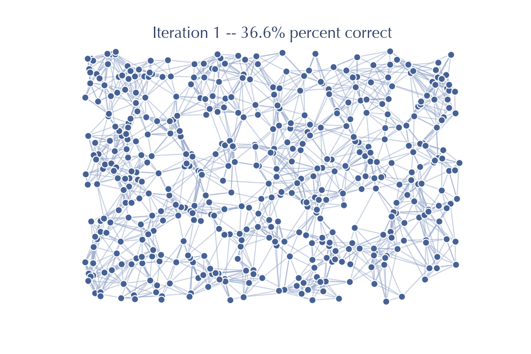
Already, after just one pass through, the graph looks a whole lot less random. And, indeed, we have already improved from the sort of accuracy of neighbors we would expect at random, to a graph that has 30% of the neighbors correct for each node (on average). That is a much better graph for doing searches on than the purely random graph, so we would expect to be able to do a lot better when we do another iteration performing updates based on friends of friends in this new much better graph.
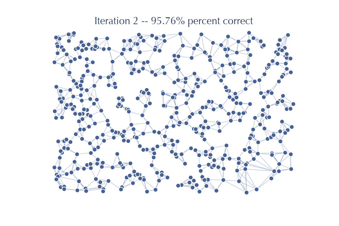
So now after just two passes we already have a graph that is 95% accurate! A search on this graph will be quite accurate, especially since we are guaranteed to be starting with a good candidate (the query itself). Running another pass should get a near perfect result.
The accuracy improved nicely, but you should note that visually there is very little difference between this graph and the previous graph. Very few edges actually changed in this iteration – the number of new neighbors, closer than any found so far, is very small. That suggests that from here on out we will get significantly diminishing returns.
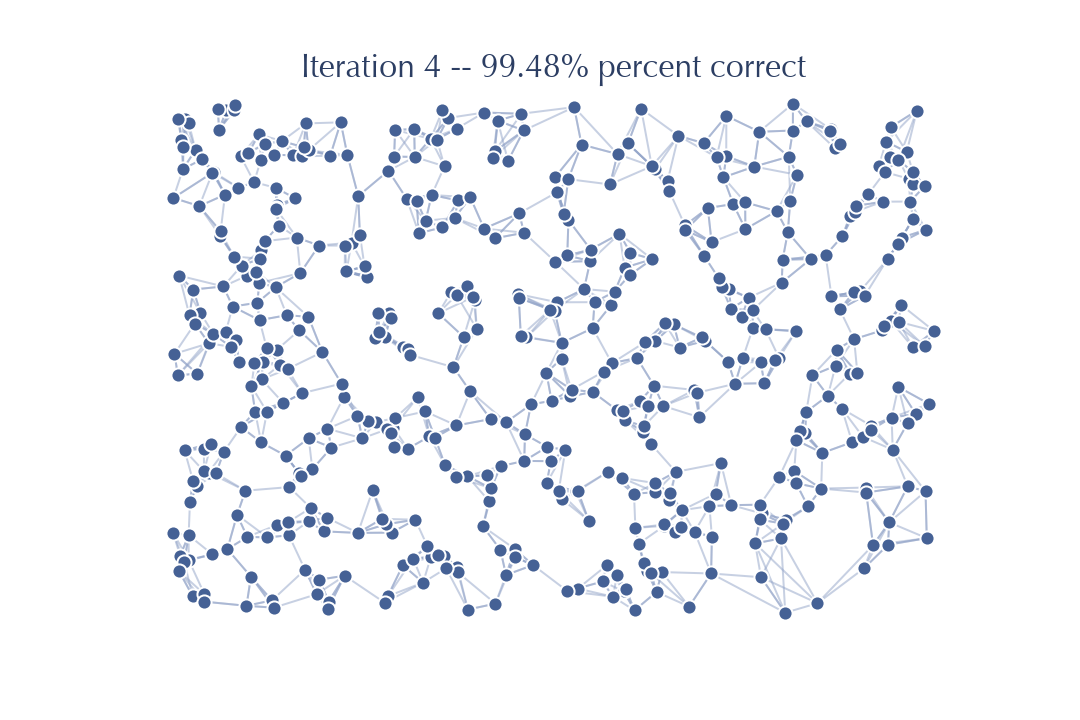
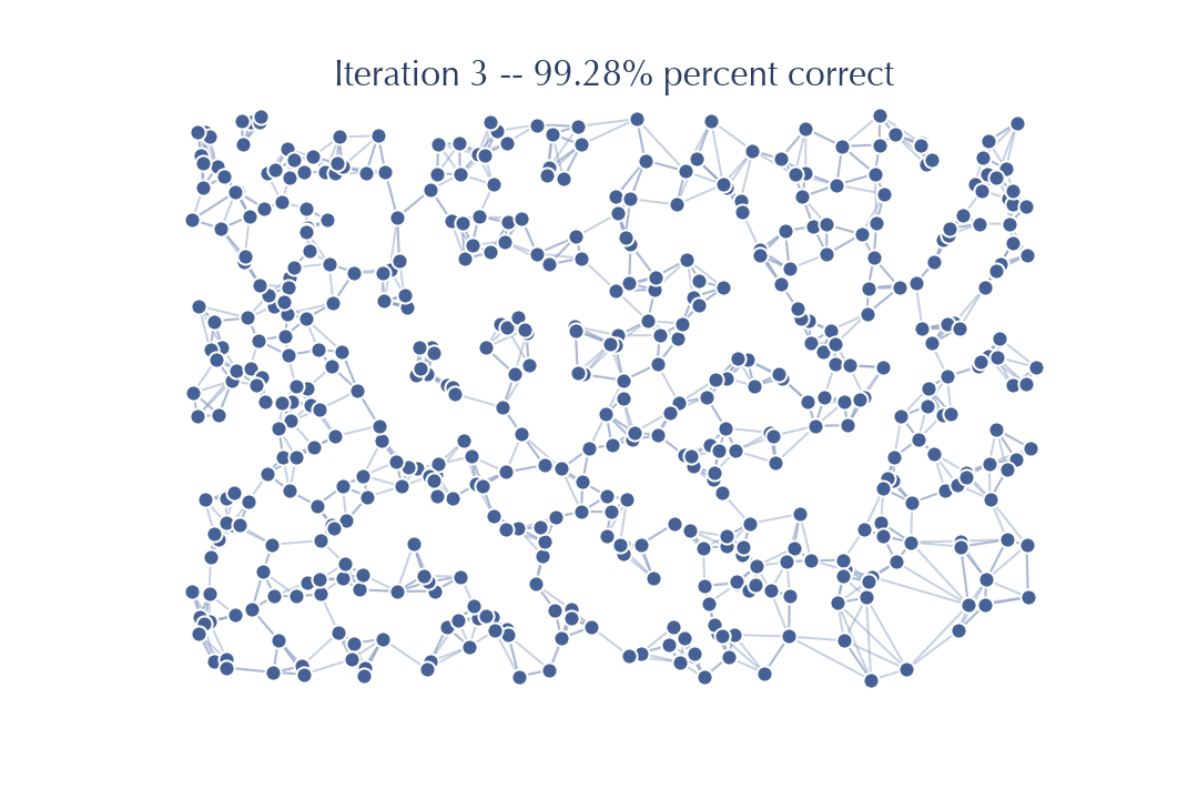
Sure enough there is little improvement this time – the last few nodes for which we do not yet have the correct \(k\) neighbors are hard to get right with a search from this graph, and so it will be challenging to make significant further improvements. Another iteration will improve things further:
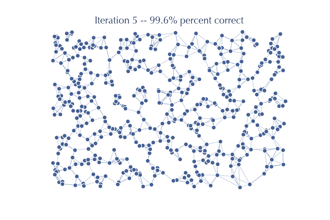
but this is where it stops. Further iterations fail to find any further improvements for the graph. We can’t get to 100% accuracy in this case. Still, 99.6% accuracy is pretty good, and will be good enough enough to be an effective search index for new previously unseen queries.
This provides us with the basic algorithm, which is already surprisingly efficient and, importantly, doesn’t rely on specific properties of the dissimilarity (such as requiring the triangle inequality) beyond the requirement that “friends of friends” should be a good source of candidate neighbors. There are a number of computational considerations that can dramatically improve practical runtime performance however. Let’s look at a few of the major ones, particularly since they involve looking at the algorithm in a different way and result in code that looks very dissimilar from what has been described so far, despite the fact that this is essentially what it is implementing.
The first major consideration is that the search should take place on an undirected graph. That means that when looking at neighbors of a node we need to consider not only the \(k\) neighbors that the node has edges to, but also all the other nodes that have our chosen node as one of their \(k\) neighbors, often called the “reverse nearest neighbors”. While it is easy to keep track of the top \(k\) neighbors for each node, it is much harder to keep track of the reverse nearest neighbors for each node, and updating that information as the graph changes becomes challenging. For this reason (among others) it becomes beneficial to compute the combined set of neighbors and reverse nearest neighbors for each node based on the graph once at the start of an iteration and use that information while updating the graph in the background. In a sense we are holding the search graph fixed for the iteration, and then applying all the updates at the end.
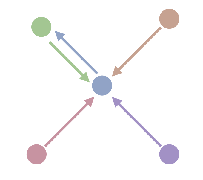
The second major consideration is a useful inversion of how we look at the problem. Ultimately for each node we need to look at the neighbors of its neighbors, which involves two hops through the graph. From the point of view of the green node we might view it as looking something like this:
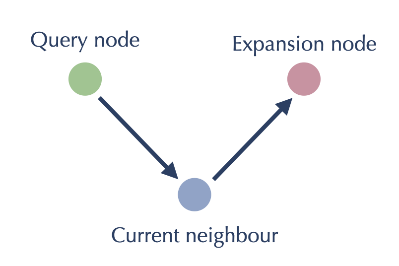
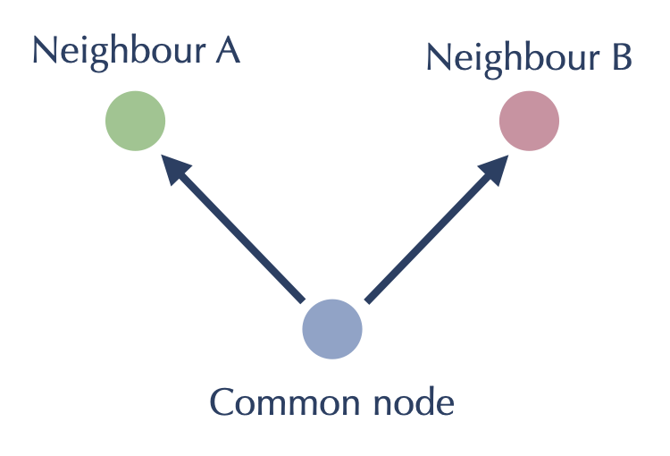
Since all our work will be on length two paths like this however, we can potentially flip our point of view around and center ourselves at the blue node. From the blue node’s point of view the goal here is have the red and the green node consider adding each other to each others \(k\) nearest neighbor lists. This flipped viewpoint saves us from some doubled work (we just need to get green and red to talk to each other at once, rather than traversing the path once from green, and then much later the other way from red), but it also turns what was a graph walking algorithm into one that is entirely local to each node: having found the sets of neighbors and reverse neighbors for every node as described above, we simply need to do an all-pairs comparison between the nodes of each such set, having each possible pairing act as the red and green nodes attached to a common node:
Putting these two considerations together we arrive at an approach that first generates a set of “neighbors” (both neighbors and reverse neighbors) for each node, then generates graph updates by doing an all-pairs distance computation on each set. After the first step of computing the reverse neighbors the all-pairs computations can all run independently in parallel, saving off the updates from each neighbor set which can then be sorted and applied to update the graph. While this is executing the same notional algorithm, viewing it this way allows for easy parallelism options, and for further efficiency tweaks: keep track of which “neighbors” are new to a set and only worry about distance computations to nodes new to the set; restrict the number of elements in the set for any iteration; exit early when the number of updates falls below a (proportional) threshold; etc.
In the end we arrive at a parallelizable algorithm that can compute an approximate \(k\)-neighbor graph of a dataset extremely efficiently. Better still it does this, much as our search algorithm did, with few constraints: we require a dissimilarity that has a “friend-of-a-friend” principle, and that the intrinsic dimension (as opposed to the apparent or ambient dimension) of the dataset is not too large. Is there any way we can speed this up at all?
Random projection trees for initialization
Random projection trees are an efficient approach to approximate nearest neighbor search for spatial data (i.e. data that has a vector space representation). The idea is simple enough: start by choosing a random hyperplane that splits the data in two (one can arrange a split by choosing two random points and taking the hyperplane to be the orthogonal hyperplane halfway between them – in either a euclidean or angular sense, depending on the distance metric); for each half choose a different random hyperplane to split that subset of the data; keep repeating this until each subset is at most some chosen size (usually called the “leaf size” of the tree). This simplistic approach manages to recursively partition up the data into conveniently sized buckets. The random hyperplanes serve two purposes: first by being at random orientations the resulting trees adapt well to high dimensional data (unlike other tree approaches such as kd-trees); second, by being randomized we can easily build many such trees that are all different. The problem with random projection trees for nearest neighbor search is that for a given query the nearest neighbors may be on the wrong side of one of those random splits, and if we just search the bucket of points in the leaf the query falls in we’ll miss those nearest neighbors. The solution is to have many trees. Since each tree is random, each tree will make different mistakes in terms of the random splits. In aggregate, by searching through a whole forest of random projection trees, the odds of finding the true nearest neighbors becomes pretty good.
So why not just use this for approximate nearest neighbor search? To get adequate accuracy one either needs to use a very large leaf size (and brute force search through all the points in a leaf), or use a lot of trees. In practice this is often much slower than the graph based search described above. Still, trees are very cheap to build, and the search can be very fast for a single tree, so can we use them somehow? Recall that we started our graph off with a random initialization, but that the better our graph was the faster each iteration ran and the better the iteration was at finding good neighbors. Could we use random projection trees to find a good starting point for the graph? It doesn’t have to be very good, just better than random. Better than random is not that hard to beat. So we can build a very small forest of random projection trees (small by the standard of the number of trees you would use if you wanted reasonable accuracy queries), and initialize our graph with it. How do we use the trees if we aren’t using them on new query points? Each leaf node of the tree is a bucket for which we can do an all-pairs distance computation, and each node in the graph can get an initial \(k\) edges based on the results of the bucket it was in. This can all be done very quickly and entirely in parallel for a small number of trees. How well does it work?
Let’s got back to our example data we built the graph for in the last section. This time we’ll use just one random projection tree to initialize things, and then proceed with nearest neighbor descent as before.
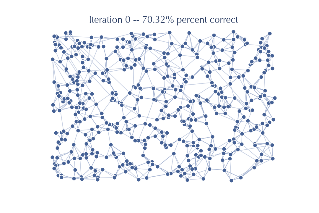
As you can see, even with only a single tree we get off to a good start; in this case 70% correct. For more difficult data in higher dimensions things won’t go this well, but as we observed above, once you have a somewhat decent graph NNDescent proceeds very efficiently:
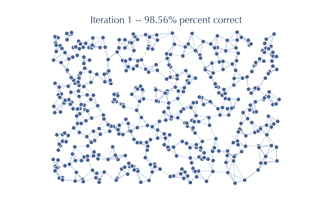
Since we started from a better graph after only one iteration of NNDescent we have already got to 98% accuracy. It takes only one more iteration of work:
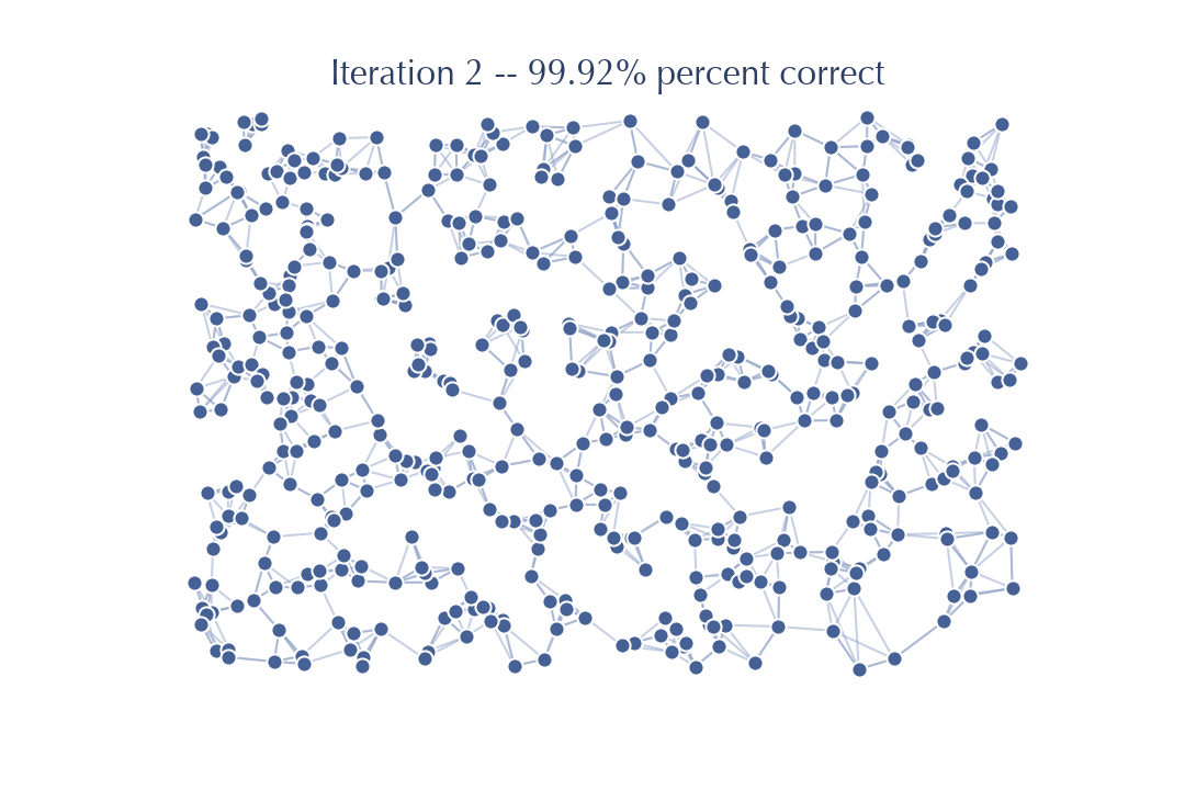
To get to a point where there are no further gains to be had. The real key is that the initialization can save us early, and very expensive, iterations. Saving a few of the early and most expensive iterations is a major gain. For this reason PyNNDescent uses a small forest of random projection trees to get a small head-start on getting a good k-neighbor graph for NNDescent to perform its iterative improvements on.
Refining the graph for faster searching
Now that we have means to build a k-neighbor graph efficiently, is there any way we can fine tune the graph to make our nearest neighbor searches run faster? One thing that slows down the search is adding lots of new nodes to the candidate pool, all of which then need to have the distance to a query point computed. If nodes have many edges attached then we end up with very large candidate pools, and search can slow significantly. While at first it seems a simple case of noting that since we built a k-neighbor graph each node has \(k\) edges, the difference is that search is conducted on an undirected graph, and this means that a node has not only edges to all the nodes that it thinks are its neighbors, but also edges to all the nodes that think it is their neighbor. For example, consider this 1-neighbor graph with five nodes – each node has a single edge to its nearest neighbor.
While each node has a single neighbor and thus a single out-going edge, if we convert to an undirected graph we end up with this situation:
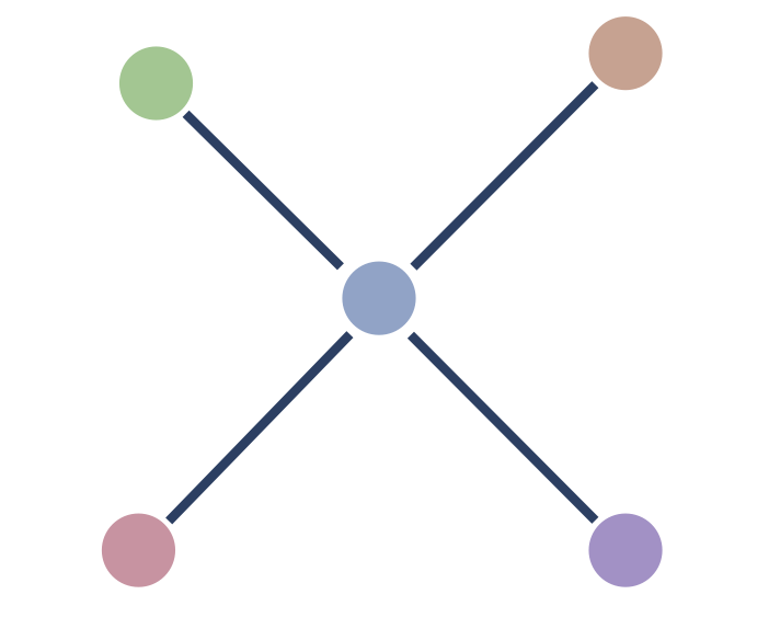
We see that the central node has four edges, despite this being a 1-neighbor graph. This can be surprisingly common, especially for high dimensional data, and the resulting undirected version of the k-neighbor graph can have nodes with orders of magnitudes more than the k edges you might expect. Pruning edges out of the graph to reduce the number of edges any one node might have attached is going to be the best way to speed up search. The catch, of course, is that removing edges can make the search less accurate. Our goal for refining the graph, then, is to remove as many edges as possible while doing as little harm as possible to the accuracy of any searches performed on the resulting graph.
One immediate possibility simply use the directed graph and throw out all the reverse nearest neighbor edges that are induced in the undirected case. While this can be effective, it does reduce the accuracy of searches; many of those reverse nearest neighbor edges are, in fact, very helpful. We could, instead, take the directed graph plus some amount of reverse neighbor edges. In cases where a node has few of these edges we can keep them all, but for the cases of nodes, such as the central node
in the example above, that have relatively many reverse neighbor edges attached, we can simply take the top few of them. This is, in fact, what PyNNDescent does using the pruning_degree_multiplier parameter. PyNNDescent will keep the top pruning_degree_multiplier * n_neighbors edges for each node, dropping any edges beyond that number.
Before we perform that kind of pruning, however, we can see if there are some other edges that we might also be able to drop with little impact on search quality. The answer is yes – specifically we can drop the long edges of triangles. What do we mean by this? Consider the case where we have a triangle formed of edges like this:
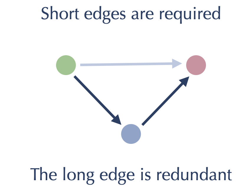
The short edges are needed to find near neighbors of each of the nodes to which they are attached. However if we follow our search algorithm we will not need the long edge since the search will traverse the two short edges and find the same result, just with one extra step / iteration. The expectation that this might slow down search doesn’t play out in practice – the gains made from removing edges dominates the small extra costs of occasionally having to take extra steps in a search. We can put together an approach to removing these long edges of triangles as follows:
For each node in the graph:
Retain the first nearest neighbor
For each other neighbor:
If the neighbor is closer to the node than it is to any currently retained neighbor, then retain it as well
If the neighbor is closer to a retained neighbor than the node, then drop it
This process ensures we keep the edges to the closest neighbors, and steadily prune out the long edges of any triangles that may occur. We can see this pictorially as follows: consider a node (in blue) with several neighbors, and suppose we have retained all the closer nodes and are considering whether to retain the green node.
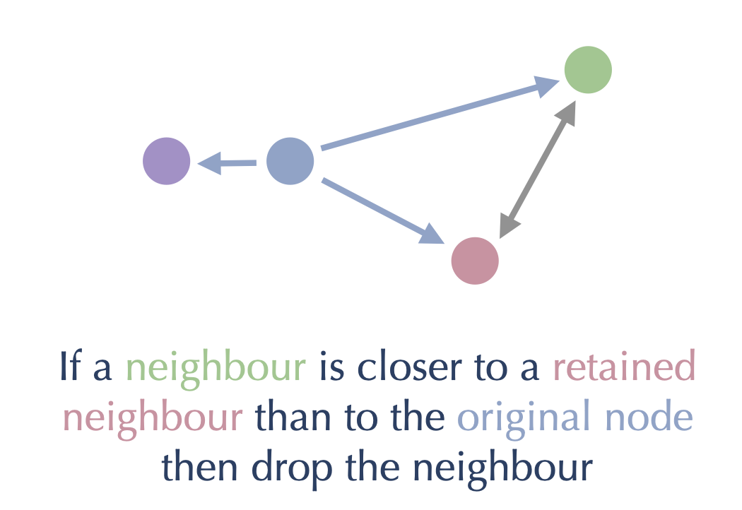
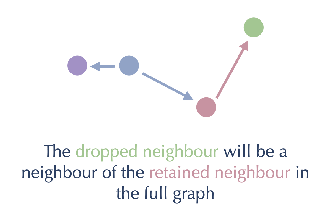
Then, since green is closer to the red node (which we already retained) than it is to the blue node we are working on, we should drop the edge from blue to green. We can get to the green node from the blue node by traversing through the red node:
By preprocessing the graph in this way, first removing the long edges of triangles and then pruning back to a maximum fixed number of edges per node, we can significantly improve the search performance on the graph. Preprocessing like this is a non-trivial amount of computational work, so by default PyNNDescent doesn’t perform that work unless specifically asked (a search query is taken to be such a request). This is because the user may be simply interested in the raw k-neighbor graph of the training data, and not in efficient querying later.
Putting it all together
We now have all the pieces in place. We can construct a k-neighbor graph using NNDescent, initialized using a small random projection tree forest. We can then refine the resulting graph to optimize it to search for near neighbors of new query points. For the search we can select a starting point using (the best) random projection tree, ensuring we start relatively near to neighbors of the query. We then the apply the graph search algorithm we started with to find the nearest neighbors of the query point. And that is how PyNNDescent works.